In economic literature, profit maximization is the primary goal of any business firm or rational producer. When we talk about the profit maximization objective, we implicitly refer to economic efficiency rather than technical efficiency. Technical efficiency does not consider the financial aspect of production; it only considers technical or engineering aspects of production, as we did in the study of production function and isoquant.
In this post, we shall examine the case of a single-product firm and discuss constrained and unconstrained profit maximization decisions facing a business firm. You can read about the case of a multi-product business firm here.
Constrained profit maximization of a single-product firm
Every producer must make a production decision regarding what to produce and how to produce it. The decision depends not only on the available production function (or technology) but also on the relative prices of factor inputs.
Due to technical and financial limitations in the short run, the producer has to make constrained profit maximization decisions with the limited resources available. In such a case, a producer can either maximize output (equally means revenue maximization given the price of a product) for a given cost outlay (financial constraint) or minimize cost for a given level of output to maximize the profit (consider a situation in which a contractor has to make a given building minimizing his total cost).
However, if a firm is new or in the long run, it does not face technical and financial limitations. It is unconstrained and free to choose the optimal way of expanding output to attain its profit maximization goal.
Two important tools—the isoquant curve and the iso-cost line—help us analyze the optimization problem. Isoquant represents the technical constraint, whereas iso-cost represents the financial constraint. For more about Isoquant, please read this.
What is iso-cost line?
The iso-cost line is the locus of all factor combinations that a product can purchase with the given outlay or budget. In other words, it shows the combinations of capital and labor that a firm can purchase with a given outlay or budget. We can present the iso-cost line mathematically as,
C = r.K +w.L
where C is an outlay, r is the rental price of capital, w is the wage to labor, and r.W and w.L are total payments made to capital and labor, respectively.
The more of the total outlay goes to labor, the flatter the iso-cost line will be and the vice-versa. And, if entire portion of outlay goes to labor than the iso-cost line reconciles with the labor axis. Similarly, the more portion of outlay goes to capital the steeper the iso-cost line will be and vice versa. If entire portion of outlay goes to capital than iso-cost line will reconcile with capital axis.
Also, I’d like to point out that a successively higher level of the iso-cost line represents a correspondingly higher level of outlay. Remaining unchanged the prices of factors, increase or decrease in outlay shifts iso-cost line parallel upwards or downwards. Similarly, remaining unchanged, the outlay and cost of one factor (say, capital) and the increase or decrease in the price of another factor (say, labor) rotate the iso-cost line, making it steeper or flatter. The ratio of factor price, w/r gives the slope of an iso-cost line.
What are the underlying assumptions?
Let us point out the main assumptions of theory:
- Objective of the firm is profit maximization.
- A modern form of production function with two variable inputs—capital and labor—is considered to apply, i.e., Q = f (K, L).
- Prices of factor inputs and products remain constant, at least during the analysis.
- Technology of production remains same throughout the analysis.
- Firm produces only a single-product.
How a rational producer minimizes outlay for given level of output?
Given the output level (or isoquant) and its price, the total revenue of the typical producer is also given as constant. For profit maximization, a producer must minimize the total cost of producing that particular good. The higher the positive gap between total revenue and cost, the higher the producer’s profit. So, the job of a rational producer here is to find the least-cost combination of factor inputs that minimize the total cost of production. A rational producer can see that the least-cost or minimum-cost combination of factor inputs maximizes his total profit by fulfilling the following two conditions:
- MRTSL,K = MPL/MPK =w/r (i.e. slope of isoquant curve = slope of iso-cost line)
- Isoquant curve be convex to origin (i.e. marginal rate of technical substitution must be diminishing)
Rearranging the terms in above equation, we get
MPL/w= MPk/r.
This is also the equivalent condition for the least-cost or optimum combination of factor inputs. That is, for the profit-maximizing least-cost combination of factor inputs, the ratio of the marginal physical product of factor inputs to its price must be the same for all factors.
Pictorial presentation of least-cost combination of factor inputs
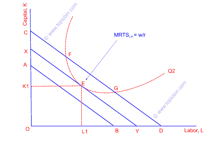
In the figure, producing at points F & G of isoquant Q2 requires a higher outlay represented by iso-cost line CD, which is an inefficient use of resources that cannot minimize the cost outlay. Meanwhile, points below the isoquant curve represent the smaller outlay, which cannot produce the given fixed level of output. This way, point E is the only possible least-cost combination of inputs, which uses the OL1 amount of labor and OK1 amount of capital to produce the given level of output Q2.
What if isoquant were concave? Producers would result in corner solutions using only one of the two-factor inputs at a lower level than before. However, our consideration is that factors are not perfect substitutes, and the marginal rate of technical substitution diminishes, which rules out the possibility of isoquant’s concave shape.
How a rational producer maximizes output for a given level of outlay?
Given the constant price of a product, output maximization equally means revenue maximization from that product. Just like the least-cost combination of inputs, a rational producer maximizes his output for a given level of outlay fulfilling the under-mentioned conditions:
- MRTSL,K = MPL/MPK =w/r (i.e. slope of isoquant curve = slope of iso-cost line)
- Isoquant curve be convex to origin (i.e. marginal rate of technical substitution must be diminishing)
The only difference here is that the producer tries to maximize output rather than minimize cost. This is only an alternative approach to the maximization problem, and the ultimate result is the same as profit maximization.
Pictorial presentation of output maximization
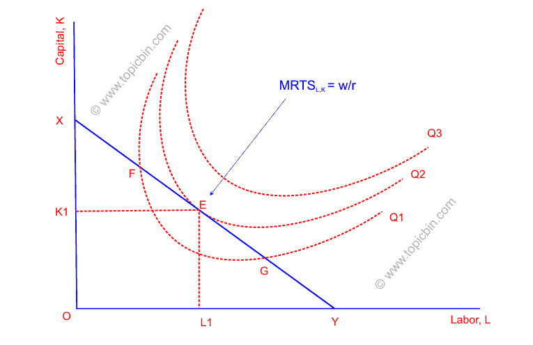
In the figure above, any points above E are desired higher levels of outputs but are unattainable because of limited outlay. Similarly, points on iso-cost line XY (other than E) or below it are undesired lower levels of output. For instance, producing at point F yields a lower output level Q1, an inefficient use of available resources. Therefore, only point E is the point of equilibrium (a profit-maximizing condition), in which the producer produces a Q2 level of output employing OL1 amount of labor and OK1 amount of capital.
Thus, in either case of profit maximization, a producer or a firm attains equilibrium (maximum profit) by employing the factors in such a way that equates the slope of the isoquant curve to the slope of the iso-cost line. In other words, the firm should use factor inputs equalizing the additional output obtainable from using another dollar on capital to the additional output obtainable from using another dollar on labor.
Unconstrained profit maximization of a single-product firm
Unlike short-run, producer does not face constraints (financial and technical) in long-run, because long-run is a time period in which everything is supposed to change. This way, a firm aims to choose the optimal path of output expansion in order to maximize the profit.
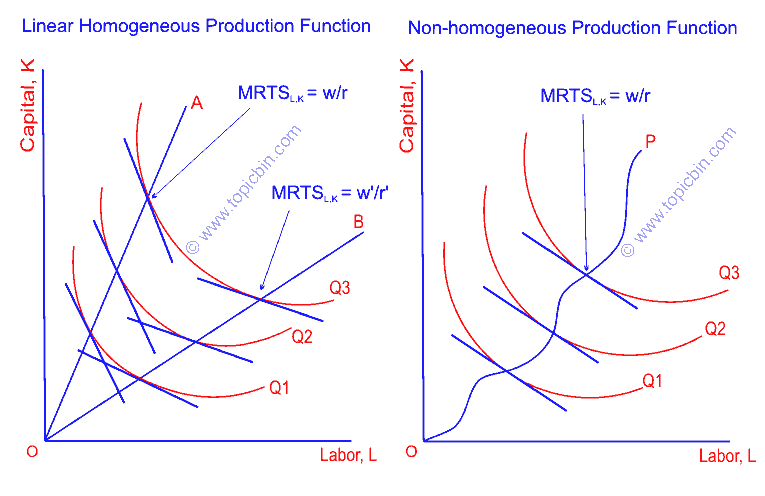
The optimal path of expansion is the locus of the point of tangency of successive isoquants and successive iso-cost lines. If the production function is linearly homogeneous, the expansion path will be a straight line passing through the origin. In the figure below, OA is the expansion path when the factor price ratio is w/r. Along the line OA, slopes of iso-cost lines and corresponding isoquants are constant. The ratio of factor prices determines the slope of the expansion path OA.
When the ratio of factor inputs increases to become w’/r’, the expansion path will be flatter OB. Likewise, a decrease in the ratio steepens the expansion path.
If the production function is non-homogeneous, the expansion path will not be a straight line. It will be a curve OP along which the equilibrium takes place equalizing the slopes of iso-cost lines and isoquants.