This article tries to explain the meaning of the isoquant curve, its assumptions, and its properties. It will also describe the marginal rate of technical substitution and the economic region of production, possibly in a detailed and obvious manner. In addition, I request you to go through the concept of production function, which will presumably ease your learning journey ahead.
Now, assuming you are familiar with the concept of production function, let’s discuss the assumptions of the isoquant curve. The main assumptions are:
- We use the production function in modern form i.e. Q = f (K, L), with only two factor inputs capital and labor.
- The technique of production remains constant.
- Efficient use of all inputs in the production of output i.e. no inputs are idle or wasted. Exactly, the production function indicates the maximum quantities of output that can be produced by employing every combination of factor inputs.
What is the meaning of isoquant?
Isoquant means equal-quantity curve; it is also called an equal-product curve. We can define isoquant as the locus of various combinations of factor inputs—capital and labor—that can produce the same or constant level of output. In other words, isoquant represents all those combinations of factor inputs capable of producing an equal quantity of output. This way, a producer is indifferent to outputs represented by various points of the isoquant curve.
Pictorial Presentation of isoquants
Let’s present the production function Q = f (K, L) in three-dimensional space to visualize what happens to output when more and more input combinations are used. By assuming the efficient use of factor inputs in production, the greater the employment of factor inputs, the greater the output it will produce. That means the production function can make the Q1 level of output using the K1 and L1 input combination. In contrast, it can produce the Q2 level of output, a greater amount of the production than Q1, using the K2 and L2 input combination as represented along the vertical output axis.
You can observe outlines of equal heights above the KL plane corresponding to the Q1 and Q2 levels of outputs. These outlines are termed elevation contours and are as equal in height as corresponding Q1 and Q2 output levels. These contours are isoquants representing the same respective levels of outputs, Q1 and Q2, that can be produced employing various input combinations in the KL plane.
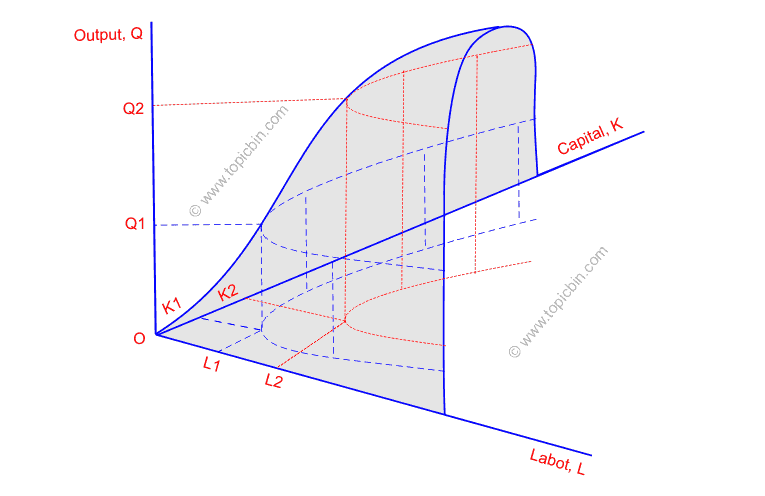
For the sake of simplicity, let us assume that these contours are projected to the KL plane. These contours – called isoquants – show various combinations of inputs that can produce particular output levels. Thus, each isoquant corresponds to a specific output level and shows technologically efficient production methods. Hence, the simplified form of isoquants will be as follows:
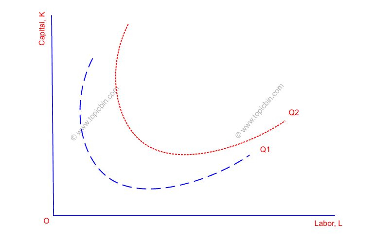
Also note, a higher level of isoquant shows a higher level of output i.e. Q2 is greater in amount than Q1. Thus, a set of isoquants can depict a production function.
What is the marginal rate of technical substitution?
The marginal rate of technical substitution is a slope of isoquant, which indicates the rate at which factor inputs can be substituted to maintain the same output level as isoquant. More specifically, a marginal rate of technical. Likewise, we can define the marginal rate of technical substitution of capital for labor, MRTSK, L, as the rate at which one unit of capital substitutes for units of labor, holding constant the level of output.
Graphically, we can present the marginal rate of technical substitution, MRTSL,K, as follows:
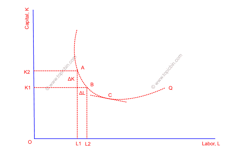
From this figure, we can observe that ΔK amount of capital has to be forgone to use an additional ΔL amount of labor i.e. MRTSL, K = ΔK/ΔL. This measurement is an arc marginal rate of technical substitution, which has measured MRTSL, K in between points A and B. Nonetheless, the point marginal rate of technical substitution of labor for capital at point C is given by the slope of the tangent at that point.
Mathematical presentation
Also following the definition of isoquant, or equal-product curve, we can write isoquant in mathematical form as
ΔKMPK + ΔLMPL = 0
or, ΔKMPK = – ΔLMPL (subtracting by ΔL *MPL on both sides)
Dividing on both sides by ΔL and MPK,
ΔK/ΔL = -MPL / MPK ……………………. (I)
Also, using the definitions of the marginal product of capital and the marginal product of labor i.e. MPK = ΔQ/ΔK and MPL = ΔQ/ΔL, we can obtain the following result,
-MPL / MPK = -ΔK/ΔL …………………….. (II)
Combining the results from (I) and (II), we get an essential relationship between the marginal rate of technical substitution and the marginal product of inputs:
ΔK/ΔL = -MPL / MPK = -ΔK/ΔL
or, MRTSL,K = -MPL / MPK = -ΔK/ΔL …………………….. (III)
The result states that the marginal rate of technical substitution equals and inversely relates to the ratio of marginal products, or productivity, of two factors.
Why does the marginal rate of technical substitution diminish?
An essential feature of the marginal rate of technical substitution is that it diminishes along the isoquant, which is called the principle of diminishing marginal rate of technical substitution. This principle implies that fewer and fewer amounts of capital are needed to use one more additional unit of labor.
The main reason behind the diminishing marginal rate of technical substitution is that the marginal product of capital increases as less capital is used, and the marginal product of labor decreases as more labor is used. Accordingly, a lesser amount of capital must be replaced by a more significant amount of labor to keep a constant output level; thus, a marginal rate of technical substitution diminishes. In rigorous terms, MRTSL, K decreases because factor inputs are of imperfect substitutes.
However, a marginal rate of technical substitution remains constant if factor inputs are perfect substitutes. In this case, the isoquant curve will be a negatively sloped straight line cutting K and L axes. The smaller the change in the MRTSL, K, the greater the degree of factor substitution. Conversely, when factor inputs are not substitutes, MRTSL, K remains infinity or zero, and isoquants become kinked and parallel to the K and L axes.
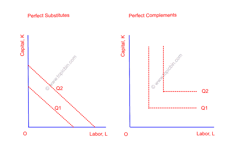
In the case of perfect complement factors, the vertical portion of the isoquant shows zero marginal product of capital while the horizontal portion shows zero marginal product of labor.
What are the possible types of isoquants?
Let’s list out the possible forms of isoquants here:
- Linear isoquant- isoquant is linear when MRTS remains constant, which happens when factor inputs are perfect substitutes. Look at the above picture of a straight line isoquant.
- Input-output isoquant – isoquant is input-output when factors inputs are perfect complements. It is also called Leontief isoquant, after Leontief, who invented input-output analysis. Look at the L-shaped isoquant in the above figure.
- Kinked isoquant is also called activity analysis isoquant or linear-programming isoquant because it is used in linear programming analysis. It is kinked because of limited factor substitutability. Thus, production is efficient only at the kinked points of isoquant. This is a discrete concept of a production function, which engineers, managers, and production executives consider to be more realistic than continuous isoquant, which traditional theory mostly adopted for ease of exposition using mathematics and calculus.
- Smooth, convex isoquant – it is continuous isoquant with a diminishing marginal rate of technical substitution and is convex to the origin.
What is meant by elasticity of technical substitution between factors?
The marginal rate of technical substitution as a measure of factor substitutability has one serious defect. It depends on the measurement unit of factor inputs, so it cannot give a true picture of factor substitutability. To circumvent this problem, another better measure of factor substitution comes into play—the elasticity of technical substitution, or simply elasticity of substitution.
The elasticity of technical substitution is the ratio of the percentage change in capital-labor ratio to the percentage change in the marginal rate of technical substitution. To say,
$$\text{Elasticity of substitution} (\alpha) = \frac {\text{Percentage change in K/L}} {\text{Percentage change in MRTS}}$$
$$= \dfrac {\dfrac {\Delta K/L}{K/L}} {\dfrac{\Delta MRTS}{MRTS}}$$
The elasticity of substitution between factors is a pure number free of a unit of measurement because both the numerator and denominator are measured in the same units that cancel out the units of measurement. Also note that when MRTS decreases, the K/L ratio also falls, and when MRTS increases, the K/L ratio also increases. This implies that the elasticity of factor substitution is positive, at least within the economic reason of production.
Where is the economic region of production in Isoquant?
One important thing to consider here is that not every input combination is economically feasible for production. Therefore, a rational producer will abandon those unfeasible input combinations unless she is compensated for their use. These unfeasible input combinations are represented by a positively sloped portion of isoquant.
A positively sloped isoquant means that a firm must use both factor inputs if it chooses to use more than one input to keep the constant level of output. Using more of one input would cause output to fall unless more other inputs were also used in production. The ultimate situation is that the marginal product of one-factor inputs is negative along a positively sloped isoquant.
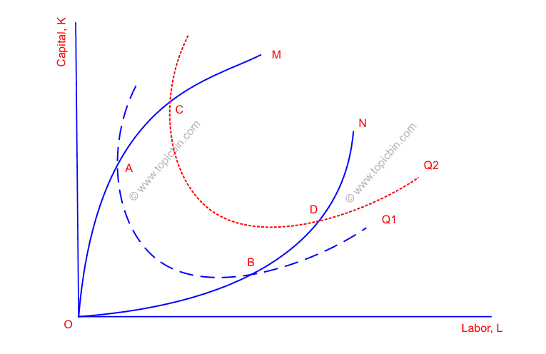
Economic region of production
In the figure, the marginal product of capital is zero at points A and C, and beyond those points (a more significant amount of capital), the marginal product of capital is harmful. Also, note that more units of labor have been used in line with capitals along the positively sloped portion of isoquant to maintain the same level of output.
Similarly, the marginal product of labor is zero at points B and D, and beyond those points (greater amount of labor), the marginal product of labor is negative. Lines such as OAC and OBD are ridge lines, which connect points on isoquants having zero marginal products. The ridge lines bound an economic region of production in which marginal products of factor inputs that are positive. Beyond the economic region of production, production is inefficient.
Factors that have harmful marginal products are called inferior factors, and we have ruled out such inferior factors in production theory unless otherwise mentioned.
What are the general properties of isoquant?
The following are the general properties of isoquants:
Isoquant slopes negatively
This is because of imperfect substitution between the factor inputs used in production. In addition, this negativity follows from the valid assumption of positive marginal product of factor inputs inside an economic production region.
Isoquant never intersects with each other
If isoquants were to intersect, it would imply different levels of outputs (at the point of intersection). A question arises: How could it be possible to produce different levels of outputs with the same input combination remaining unchanged in the production technology? This is against the fundamental assumption of isoquant.
An isoquant is convex to the origin
This is because of the diminishing marginal rate of technical substitution of factor inputs. Likewise, the diminishing marginal rate of technical substitution will come into effect because of the imperfect factor substitution, which is again the result of the operation of diminishing marginal returns of factors. If isoquant were to concave, it would indicate increasing returns. However, diminishing returns are more accurate in the real world. Thus, we could assume a diminishing marginal rate of technical substitution and, accordingly, isoquant convex to the origin.
One problem with concave or straight-line isoquants is that the producer’s equilibrium results in a corner solution. A corner solution is where employment is the only factor input in production. However, in reality, more than one factor is used in production. Hence, it is rational to have isoquants convex to the origin.