If you are a beginner and have just started to study production theories of microeconomics, you are in the right place to start from. After studying this article, you will learn the concepts of production, production function, and total, average, and marginal product and their relationships. Moreover, you will also get to know types of production functions based on time, variability of factor proportions, and factor substitutability (linearly homogeneous production function, Cobb-Douglas production function, and CES production function) in a clear-cut way.
The theory of production is a very crucial subject matter in the field of economics. Production theories heavily rely on the concept of production and the production function. Therefore, let’s understand what production and the production function are. In this scenario, the sections mentioned below try to elaborate on these concepts one after another.
Concept of Production and Production Function
In the economic profession, production refers to the creation of utility. The creation of utility is possible through converting factor inputs into output, and the production function does this job. Inputs used in production are factors of production or, simply, factor inputs. The production function incorporates factor inputs in the production process and yields the output. Hence, the production function is the process that converts the inputs into output. In other words, the production function is the technical or engineering relationship between factor inputs and outputs. Let’s express the production function mathematically as follows:
Q = f (K, L, M, N, …, Z) … … … (I),
Where ‘f’ denotes the functional relation between output, Q, and other factors of production like capital, labor, land, raw material, energy, entrepreneur, technology, and so on.
However, in modern economics, labor and capital are the only two dominant factors of production. Economists overlook other factors of production to produce a basic economic framework or economic model with ease of exposition. Accordingly, the usable production function shall revert to
Q = f (K, L) … … … (II),
Where notations stand for their usual meaning, and K and L are exogenous variables, i.e., their values are taken as given. Unlikely, Q is called endogenous, i.e., whose value depends on other variables and varies over time. In addition, the production function also represents the technology of production equally. The basic economic theory of production assumes only the efficient production method because a rational producer will not use an inefficient production method.
Total, Average, and Marginal Concepts of Production
We need some preliminary concepts while studying the production theory. They are total products and per-unit products. The total product of capital (TPK) and the total product of Labor (TPL) are the total product concepts. The marginal product of capital (MPK), the marginal product of Labor (MPL), the average product of capital (APK), and the average product of Labor (APL) are the per-unit product concepts. We elaborate on these concepts in terms of labor, which applies equally to capital as well.
Total Product
The total product of labor is the aggregate output produced by the total labor units used in the production. Alternatively, TPL is the sum of marginal products of labor, i.e., TPL = MPL (1) + MPL (2) + MPL (3) + … + MPL (n-1) + MPL (n), where MPL (n) is the marginal product of labor from an nth unit of labor.
Average Product of Labor
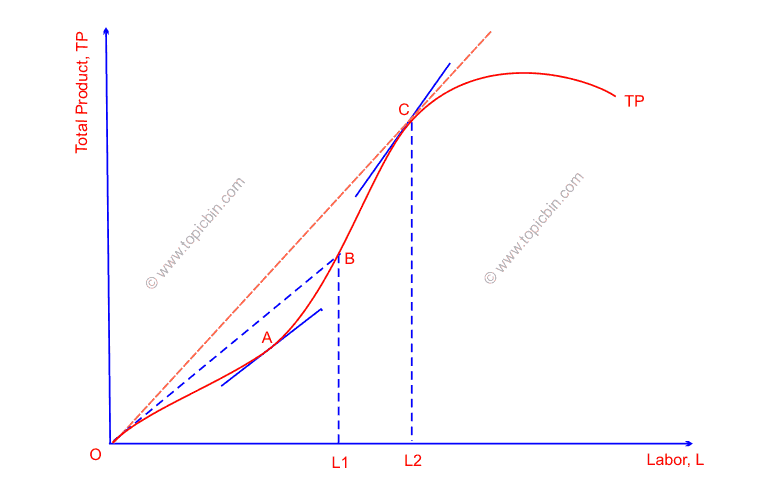
Dividing the total product of labor (TPL) by the total number of laborers (L), i.e., APL = TPL /L, results in the output per unit of labor (APL). In the figure below, the slopes of line segments OB and OC give the average products of labor at points B and C, respectively.
Marginal Product of Labor
It is the extra unit of output produced by employing one additional unit of labor. Put another way, it is the change in TPL due to a change in one extra unit of labor, i.e.
MPL= ΔTPL / ΔL
Where Δ shows the change in the respective variables (ΔL is always one because labor units change one by one, i.e., 1, 2, 3… n-1, n persons). This is a per-unit production because the marginal refers to the yields from the one additional factor unit. That means we are talking about calculating marginal product from tabular data (also called discrete data), and such calculation of marginal product is called arc marginal product because it measures marginal product between two points. However, the following figure measures point marginal product of labor at points A and C, given by the slope of respective tangents, as they measure the marginal product at those points.
Graphically,
Relationship between MPL and TPL
When MPL keeps on increasing, TPL increases at an increasing rate; when MPL remains constant, TPL increases at a steady rate; when MPL decreases, TPL increases at a decreasing rate; when MPL is zero, TPL remains constant; and when MPL is negative, TPL decreases.
Relationship between MPL and APL
When MPL > APL, APL increases; when MPL = APL, APL remains constant; when MPL < APL, APL decreases.
In the subsequent section, we will examine the types of production functions.
Long-run vs Short-run Production Function
What separates the long run from the short run in the economic profession? The answer is undoubtedly the time a variable takes to vary. In this regard, factors of production are classified into long-run and short-run based on variability, i.e., the time they take to vary. This classification is beneficial for examining and understanding the theories of production thoroughly.
In economics, a short run is a time interval in which we cannot even change a single factor input. Thus, if at least one factor input is unchangeable during the period, then a production function is short-run. In other words, when not all factors of production are variable, then a production function is short-run and called a short-run production function. Hence, the short-run production function must fix at least one factor input.
On the other hand, all the factor inputs are variable in the long-run production function. The long run is the period in which all factor inputs included in the production function can be changed. However, no specific law stipulates the short- and long-run. It is all about the theory, but in practice, it depends on the nature of production activity that determines short- and long-run. That is why the practical thinking of economists is that the long run is a planning period in which decisions regarding investment in new plants and machinery can be undertaken. In contrast, the short run involves the operations of existing plants and machinery.
Fixed vs Variable Proportion Production Function
Let us first understand the concept of proportion before starting the topic. Proportion refers to the equality of two ratios; that is, connecting two ratios by an equality sign results in a proportion. In this way, ratios are integral parts of proportion, and we mean proportion here to refer to the equality of different capital-labor ratios.
Another thing to consider here is a term called technical coefficients of production, which is the amount of factor inputs required to produce a certain commodity. For example, suppose that 10 units of capital are needed to produce 50 units of a particular commodity; then, the technical coefficient of capital for production is 0.2. If we were to express it on a percentage basis, it would require 20 percent capital to produce 50 units of the commodity.
Now that we have defined the proportion and technical coefficients of production, it is time to describe fixed and variable proportion production functions. Whether the production function is variable or fixed proportion depends on the technical coefficients of production. If the technical coefficients of factors are constant, then the production function is a fixed or constant proportion production function; otherwise, it is a variable proportion production function.
In a fixed constant proportion production function, the capital-labor ratio remains fixed no matter how large the production scale is, as opposed to a variable proportion production function. Likewise, there is zero marginal rate of technical substitution between factor inputs -capital and labor- in a fixed or constant proportion production function, which means factors are perfect complements. On the other hand, there might be limited factor substitutability or perfect substitutes in the case of a variable-proportion production function.
Linearly Homogeneous Production Function
The production function is homogeneous of degree r if the multiplication of each factor input of a production function by a constant ‘j’ leads to the multiplication of output by jr.
Mathematically, the general homogeneous production function of degree r is written as:
jr Q= F(jL, jK) where j, r > 0 …………………. (III)
where Q is output, L is labor, K is capital, and j and r are constants greater than zero. However, j and r can take any value, but we take these values as positive from the perspective of economic variables, which are rarely negative.
When the value of r in equation (III) is 1, the homogeneous production function is of first degree, which is also the linearly homogeneous production function we refer to. That means jQ= F(jL, jK) is a linearly homogeneous production function, and it implies that multiplying factor inputs by a constant j results in multiplying output by the same constant j. Thus, it shows constant returns to scale.
Characteristics of Homogeneous Production Function
General homogeneous production function jr Q= F(jL, jK) exhibits the following characteristics based on the value of r.
If r = 1, it implies constant returns to scale. In such a case, the production function is said to be linearly homogeneous of the first order.
If r > 1, it implies increasing returns to scale.
If r < 1, it implies decreasing returns to scale.
Due to its simplicity and good approximation of real-world situations, linear programming and input-output models widely use this production function.
Cobb-Douglas Production Function
This very famous Cobb-Douglas production function is a long-run production function. It is the result of the combined efforts of Professor of Economics cum U.S. Senator Paul Douglas and mathematician Charles Cobb. Douglas observed U.S. data and found that the shares of national income to labor and capital remained almost constant over the long period. Put another way, despite continuous growth in national income, the proportionate share of labor and capital in national income nearly grew constantly. The special case of the Cobb-Douglas production function depicts this fact.
Mathematical representation of the general Cobb-Douglas production function is as follows:
Q= F(L,K) = A Kα Lβ where A, α, β > 0 …………………. (IV)
where Q is output, α is output elasticity of capital, β is output elasticity of labor, and A is productivity, or total factor productivity, measuring the productivity of the production function or technology or factor inputs in total. All of these parameters are positive. If the production technique advances, it raises the value of the productivity parameter, A. Raising the value of total factor productivity, A, equally means that the productivity of both labor and capital has increased.
The parameters α and β, which also measure the shares of national income to capital and labor, are distribution parameters. That is, parameters α and β measure the contribution of capital and labor to total production or national income. Note that the usage of the Cobb-Douglas production function here is in a macro sense. For this reason, it is often called an aggregate production function. However, it can be used in the micro sense as well.
Characteristics of Cobb-Douglas Production Function
Let’s observe the Cobb-Douglas production function Q = A Kα Lβ, supposing that we change capital and labor by some constant multiple of λ, which results in the right side of the function as:
A (λK)α (λL)β = λα+β A Kα Lβ = λα+β . Q
This implies that by increasing the factor inputs by a multiple of some constant λ, output increases by the multiple of λα+β. That means the coefficient λα+β shows the joint contribution of capital and labor to output. More specifically, coefficient α+β is a measure of returns to scale. You can find more information on the law of returns to scale.
If α+β = 1, it implies constant returns to scale. In such a case, the production function is linearly homogeneous of first order.
If α+β > 1, it implies increasing returns to scale.
If α+β < 1, it implies decreasing returns to scale.
In the case of a linearly homogeneous production function of the first order, the following features hold:
- Cobb-Douglas production function exhibits constant returns to scale. That means doubling the factor inputs doubles the output by the same proportion.
- It demonstrates diminishing returns, i.e., the marginal product of the factor diminishes. More precisely, the more and more usage of factor inputs leads to the decreate in its marginal productivity, holding the other factor inputs constant.
- It exhibits the unit elasticity of factor substitution (For more read here).
Initially, the manufacturing industry used the Cobb-Douglas production function. Empirical studies widely use it nowadays.
CES Production Function
CES stands for constant elasticity of substitution. This latest CES production function is due to the joint effort of Arrow, Chenery, Minhas, and Solow. This CES production function is a more general production function that yields constant elasticity of factor substitution other than 1.
Mathematically, the general CES production function is written as:
Q= A[?K-ρ + (1-?)L-ρ]-1/ρ where A > 0, 0<?<1, -1<ρ≠0 ………………. (V)
Where Q is output, L is labor, K is Capital, and A is the efficiency parameter serving as a state of technology. As A is a distribution parameter showing relative factor shares, α and β are the function parameters in Cobb-Douglas production; ρ is the substitution parameter that has no counterpart in the Cobb-Douglas production function and is a determinant of constant elasticity of substitution in the CES production function.
The elasticity of substitution between factors (σ) is given by 1/(1+ρ) in the CES production function i.e. σ = 1/(1+ρ).
Characteristics of CES Production Function
CES production function is linearly homogeneous and exhibits constant returns to scale. Based on the value of ρ, it produces the following results for σ :
When -1<ρ<0, then σ >1.
When ρ = 0, then σ = 1.
When 0< ρ < ∞, then σ < 1.
Cobb-Douglas production function is a special case of the CES production function when there is unitary elasticity of substitution. This means that the linearly homogeneous CES production function is a Cobb-Douglas production function producing constant returns to scale.