This article explains the law of variable proportions. You will learn the core concept of this famous production theory in economics. Before reading this article, we recommend that you read through the fundamental concepts regarding production and the production function, which will facilitate your learning going forward.
Since you studied the recommended article, I guess you know the fundamental concept of the production function very well. Let’s proceed with the theory.
For the sake of simplicity, we assume that the production function consists of only two-factor inputs—labor and capital. Accordingly, the production function turns out to be Q = f (K, L), which includes only two factors—K and L—by dropping out other factors. This is because K and L are the dominant input factors, simplifying the theory’s explanation and graphical presentation.
Holding at least one factor input constant, ideally capital, means that the law of variable proportions is associated with the short-run production function. As a result, we assume the production function Q = f ($\overline{K}$, L), where $ \overline{K}$ is a fixed factor in the short run.
Assumptions of Theory
- Technology remains fixed.
- At least one factor (capital in our case) must be constant.
- Factor inputs (as we have assumed labor and capital) are not perfect substitutes.
- Variable factor (labor) is homogeneous.
Statement of Theory
The theory states that when the variable factor (labor) is employed more and more with the given fixed factor (capital), the total product of labor (TPL) increases at an increasing rate in the early stage of production; after a certain point, the total product of labor increases at a decreasing rate, reaches a maximum, and starts to decline. In brief, when more units of variable factor are successively used with the fixed factor, the marginal product of labor eventually decreases. This is why this theory is also known as the law of diminishing returns (or diminishing marginal productivity). This way, the law of variable proportions shows how output changes when more and more variable inputs are used with a constant amount of fixed factor.
Explanation of theory
Let us explain the theory with a numerical example. Given the fixed 5 units of capital, suppose the number of labors and corresponding outputs as follows:
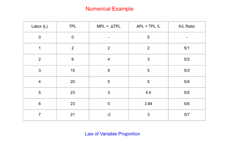
In the table given above, the total product of labor increases at an increasing rate up to the third unit of labor because the marginal product of labor increases up to the third unit. After the third unit, the total product of labor increases at a decreasing rate because the marginal product of labor has started to decline thereafter.
However, the average product continues to rise and reaches a maximum when the average product is increased, and the marginal product decreases to equal the fourth unit. After the third unit, the marginal product decreases faster than the average product increases. Hence, the average product also declines after the fourth unit but never touches the horizontal axis.
Likewise, the marginal product of labor continuously decreases to zero at the 6th unit, at which the total product reaches its maximum. After that, the marginal product becomes negative after the 6th unit. Accordingly, the total product starts to decline, reaching its maximum at the 6th unit. Also, the K/L ratio changes as labor changes, given the fixed capital; hence, the name of this theory is the law of variable proportions.
Pictorial presentation
This numerical value in the table can be shown graphically as follows:
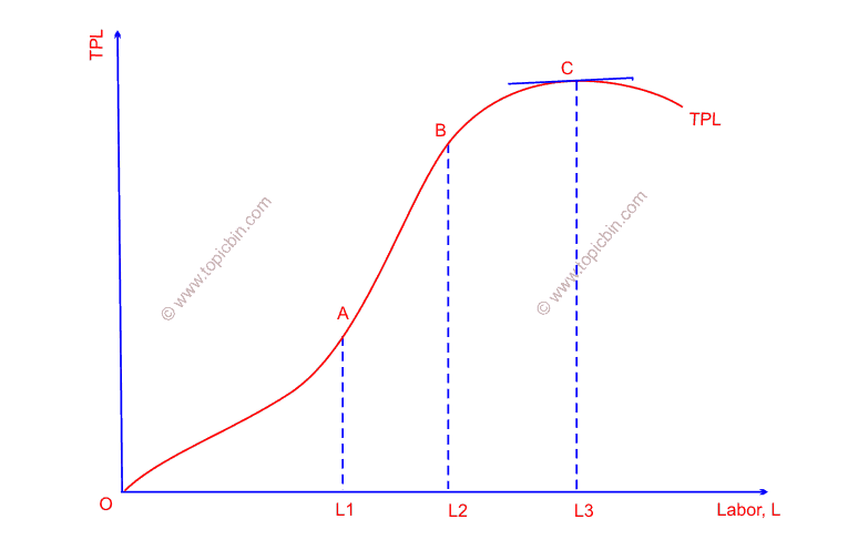
Initially, the shape of the TPL curve is convex to the origin. The convex shape results from the negative marginal productivity of the fixed factor (capital) (why?), which turns out to be positive with more variable factors. After a certain period, the TPL curve is concave to the origin because of the diminishing marginal product of labor. There are three stages of production: first, second, and third. We will explain each of them as follows:
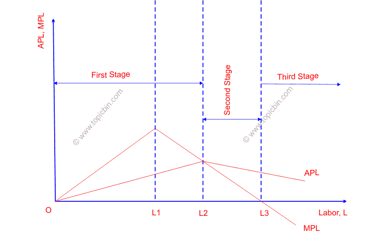
First stage:
This production stage is the stage of increasing returns because the average product rises and reaches the maximum when the marginal product equals the average product, despite the marginal product having already begun to decline. Hence, the first production stage goes from zero units to 4th, i.e., L2 labor units. The first stage ends with the start of the fall of APL. The leading causes of the increasing returns are the fuller and more efficient utilization of fixed factors and specialization of labor.
Second stage
This stage of production is diminishing returns because both average product and marginal product decline but remain positive throughout this stage. Thus, the second stage starts with the fall of the average product and terminates when the total product reaches maximum (when MPL is zero). This second stage lies between L2 and L3 labor units, as shown in the figure. At this stage, output increases at a decreasing rate because of decreasing marginal product. Nonetheless, APL keeps on rising until marginal product equals average product.
The main causes of diminishing returns are the excess of a variable factor over the fixed factor, the indivisibility of the fixed factor, and no perfect substitution between factor inputs. Prof. Bober rightly remarks on indivisibility: “Let the indivisibility enter through the door. The law of variable proportion rushes out through the window.” In addition, a scarce factor is taken as the fixed factor, and its supply cannot be increased. Also, the factors are not perfect substitutes by assumption.
Third stage:
This is the stage of negative returns because of the negative marginal product of labor. The total product declines in this stage due to the negative marginal product of labor. However, the average product remains positive so long as the total product is positive. The leading causes of the negative returns are excess variable (labor) over the fixed factor (capital) and difficulty in management and control. This situation is rightly underscored by the proverb – “too many cooks spoil the broth.”
Stage of operation for a rational producer
A rational producer never produces at the third stage because, in this stage, the marginal product is negative and reduces the total product. Cutting the number of laborers would provide the producer with more output. Hence, the third stage is not the stage of operation for a rational producer. Similarly, a rational producer does not produce at the first stage because, at this stage, the marginal product of the fixed factor (capital) is negative. Increasing the variable factor means the fuller and more efficient use of the fixed factor. Hence, the producer does not produce in the first stage. The only remaining stage of operation is the second stage.
A rational producer operates in this stage because the total output increases despite decreasing average and marginal products. Hence, a rational producer operates somewhere between the 4th and 6th units. But the exact point at which the producer operates depends on the relative price of the factors.
Application of the law of variable proportion
Initially, the law of variable proportions was considered to operate only in agricultural production. However, this law has vast and universal applicability and applies to agriculture and industry sectors. Moreover, the application of diminishing returns means that the future of individuals looms large as a gloomy picture. Starvation, underproduction, shortage, hardships, misery, and so on might happen due to continual productivity decline.
Nonetheless, why are we not observing these dismal situations universally in the real world? The answer lies within the assumption of ‘other things remaining the same’. That means we have assumed the production technique to remain constant throughout the theoretical analysis. However, technological advancement is a continual process that keeps developing, ultimately contributing to higher productivity growth.
In a nutshell, we can suspend diminishing returns through continually advancing production techniques.