The purpose of this article is to teach you about the different versions of the quantity theory of money, along with underlying assumptions and flaws. Italian economist Davanzatti developed the quantity theory of money, and American economist Irving Fisher popularized it after his influential book “The Purchasing Power of Money” in 1911.
Statement of Theory
This theory postulates a direct and proportional relationship between money supply and price level and an inverse and proportional relationship between money supply and the value of money (1/p). In terms of Fisher, “Any given percentage increase or decrease in money supply will lead to the same percentage increase or decrease in the general level of prices.”
Assumptions
- The price level is a passive variable i.e. money supply determines the price level.
- People use money only as a medium of exchange. That is, people do not hold money as idle cash balances. Holding idle cash means foregoing the interest earnings that could be earned by keeping in savings deposits and investing in securities. Even if people hold money, they have it for transactions only. Hence, people spend all their accumulated money either on consumption or on capital goods. Thus, all the money supplied is in circulation.
- There is always full employment in the economy i.e. economy utilizes all resources fully.
- The volume of goods and services, and the velocity of money remain constant in the short run.
- The supply of M1, credit money, depends on M and the ratio of M1 to M remains the same.
Equation of Exchange
Fisher had given the equation named ‘Equation of Exchange’ to explain the quantity theory of money as
MV = PT
where,
M = money supply (currencies and notes in the hands of people),
V = transaction velocity of money. It is the average number of times that a currency passes through hands or changes hands during a specific period, especially a year,
P = general price level i.e. average price of goods and services, and
T = total volume of transacted goods and services.
Example of Velocity of Money: Suppose that a ten-dollar bill changes hands five times to purchase 5 pieces of journals costing $10 each during a year. Then, M, V, P, and T equal 10, 5, 10, and 5 respectively.
The value of V is associated with the nominal value of total transactions in an economy. This is whyV is transaction velocity. Fisher assumed that the velocity of money depends on institutional and technological features (such as spending habits and the introduction of debit cards) in the economy, which change only gradually. So, the velocity of money remains constant in the short run.
Similarly, T is constant because there is full employment in the economy and the economy utilizes all resources – labor and capital- fully. In addition, the output of an economy depends on the aggregate production function (technology) and the quantities of factors of production available. Thus, the output is constant in the short run because factors like technology, capital, and labor are constant in the short run.
Revised Version of Equation of Exchange
Later on, Fisher revised the ‘equation of exchange’ to include bank or credit money because of their increasing importance in later periods. Thus, the revised equation is MV + M1V1 = PT.
Where M1 is the credit or bank money, and V1 is the velocity of the Credit Money. Note that the assumption of a constant ratio of M1 to M validates this form of ‘equation of exchange’ as well.
Quantity Theory of Money
Given the constant V and T, an increase or decrease in the money supply (M) leads to a direct and proportional increase or decrease in the price level P. For example, a 10 % increase in M leads to a 10% increase in the price level and a 10% decrease in the value of money (1/P).
The assumption of constant V over a long period transforms the equation of exchange to the quantity theory of money. This theory states that the quantity of money solely determines the economy’s nominal income (spending). Doubling the money supply (M) doubles nominal income (Py) (see Cambridge version below).
Tabular Presentation
Consider the following hypothetical example:
| Money Supply (M) |
Price Level (P) |
Value of Money (1/P) |
| 1000 |
2 |
0.5 |
| 2000 |
4 |
0.25 |
| 4000 |
8 |
0.125 |
| Given, V=5 and T= 2500 |
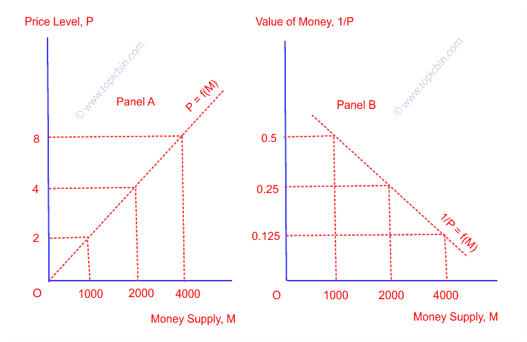
The table shows that doubling the money supply has doubled the price level, but the value of money has declined by half. Notice that all these changes are proportionate in that each change by 100%.
Graphical Presentation
 Quantity Theory of Money
In the figure above, increasing the money supply by 100%, i.e., from 1000 to 2000, the price level also has increased by 100%, i.e., from 2 to 4 (Panel A). At the same time, the value of money (1/P) decreased by 100%, i.e., from 0.5 to 0.25, as shown in panel B. A similar situation has occurred when the money supply is doubled from 2000 to 4000. Hence, the figure shows the direct and proportionate relationship between money supply and price level, but the inverse and proportionate relationship between money supply and value of money.
Cambridge Version of Quantity Theory of Money
Cambridge University’s economist Marshall transformed the ‘equation of exchange’ in this Cambridge version. Due to the double counting problem and difficulty measuring the nominal value of the total number of transactions in an economy, measuring T in Fisher’s equation became impractical. Thus, Marshall revised Fisher’s equation to include only final goods and services, y, in place of T.
Accordingly, the transaction equation of exchange turns out to be MV = Py,
where y is final goods and services or aggregate output, and V is the income velocity of money. The income velocity of money is the average number of times a dollar is spent per year. Moreover, V is the income velocity of money instead of the transaction velocity because the total nominal income of an economy, Py, comes into play instead of the total transaction, PT.
This Cambridge version of the Quantity Theory of Money establishes the connection between a country’s total nominal income and total money supply. Here, total nominal income refers to the total amount of spending on final goods and services in an economy within a year. Given the constant V and y, the equation of exchange states that the quantity of money multiplied by its velocity must equal nominal income. This analogy implies that a proportionate change in money supply leads to a proportionate change in price level.
The equation of exchange can be written as M =1/v (Py) or M = k (Py), where k = 1/v. The right-hand side of the equation, k(Py), is the demand for money, and the left-hand side, M, is the money supply. The money market will be in equilibrium when money demand equals money supply.
Monetary Neutrality
As we just outlined, the money supply only affects the price level. Quantity theory shows that money is neutral. The phenomenon that the money supply does not affect real variables is called monetary neutrality.
Implications of Quantity Theory of Money
Let us present the following implications:
- Price Level – the changes in the quantity of money lead to directly proportionate changes in the price level.
- Inflation – the quantity theory of money, the theory of inflation states that inflation is the difference between money supply growth and aggregate output growth. The justification rests upon the mathematical fact that the percentage change of a product of variables is approximately equal to the sum of percentage changes of individual variables. Accordingly, we can write an equation of exchange as,
%change in M + %change in V = %change in P + %change in y
Since V is constant, the percentage change is zero. So, %change in P (inflation) equals
%change in P = %change in M – %change in y.
- Real income – On the one hand, classical economists believe that wages and prices are flexible enough to restore the economy to the full employment level of equilibrium. You can read Say’s Law of Market for the justification provided by classical economists. On the other hand, the full employment level of output depends on the economy’s aggregate production function and the quality of available resources. Both of these facts imply that changing money supply leads to directly proportionate change in price level and, thus, nominal income, but it does not alter the real aggregate output because there is a full employment level of output in the economy. This implies a complete separation between nominal and real variables like money, income, wage, and interest rate. Classical economists term this separation as a classical dichotomy.
Flaws or Criticisms of Quantity Theory of Money
- Price is not a passive factor but it is active because price tends to encourage the producer to produce more. The higher price is the incentive for the producer to produce more.
- People hold money not only as idle cash to meet their daily liquidity needs but also for precautionary motives.
- There is not always full employment in the economy but less than full employment.
- The value of V may rise during the boom period and fall during the recession period. So, we cannot expect the value of V to be constant.
- The price level and value of money may not change proportionately to the money supply.
If you like this article, then also don’t miss to read Say’s Law of Market, another pillar of a complete classical model.